16 ARIMA Models
16.1 Introduction
In the previous two chapters, we introduced the key characteristics of time series data and reviewed the importance of identifying (and dealing with) stationarity in time series data.
In this chapter, we’ll explore how we can work with time series data to build predictive models.
We focus on ARIMA (AutoRegressive Integrated Moving Average) models and how they can be used for analysing and forecasting time series data.
Alternatives to ARIMA, which we won’t consider in this module, include State-Space models (such as Kalman Filters).
16.2 ARIMA Models
An ARIMA model is a statistical method used for forecasting time series data; data points collected over time.
It’s a way of building predictive models based on historical time series data.
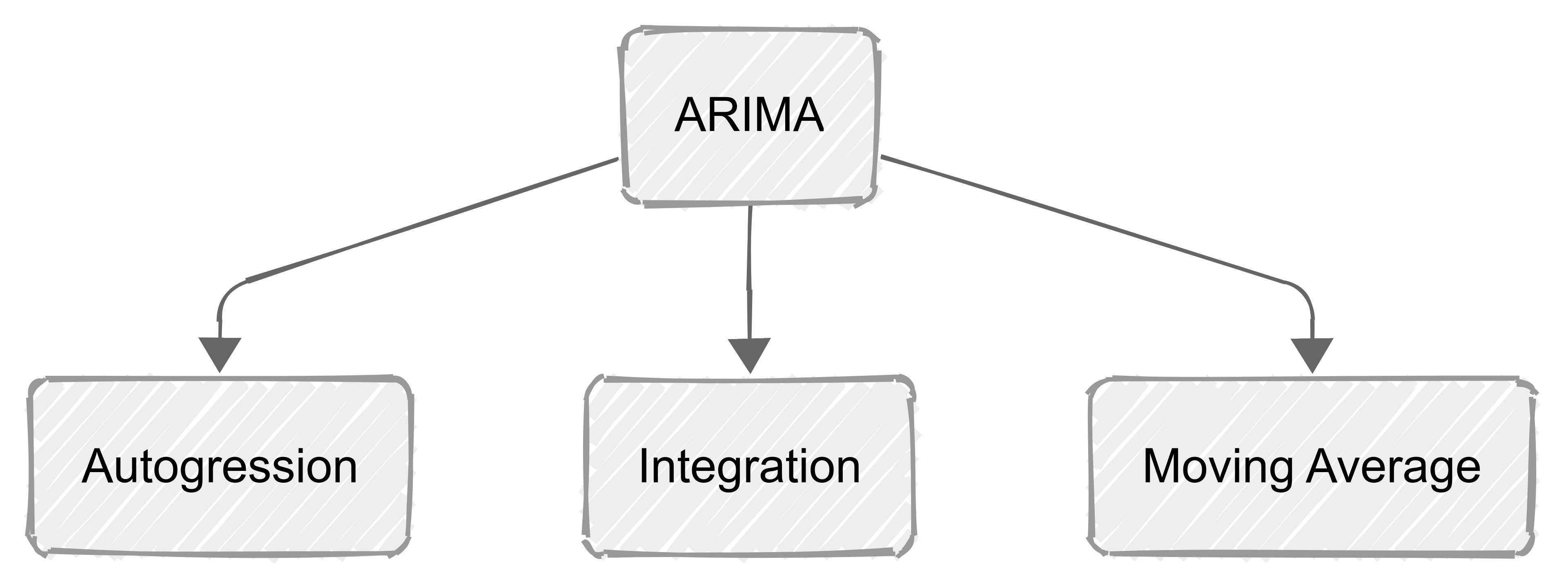
ARIMA models combine three key components:
autoregression (AR), which captures the relationship between an observation and its previous values;
integration (I), which addresses the need for differencing to make the series stationary; and
moving average (MA), which incorporates the dependency between an observation and past residual errors.
ARIMA models help us predict future points in series by examining the differences between historical values, instead of through direct values.
This makes them particularly effective for non-stationary data that have been made stationary through differencing (see previous chapter).
16.2.1 Terms in ARIMA models
ARIMA models contain three terms (components): \(p\), \(d\), and \(q\):
\(p\) is the number of autoregressive terms (AR). It represents the number of lags of the dependent variable included in the model.
- For example. an AR(1) uses the previous time step to forecast the current one.
\(d\) is the order of Integration. This determines how many times the data have been differenced to achieve stationarity (see previous chapter).
- If there is a trend in the data we might need to difference them once. therefore d = 1.
\(q\) is the number of moving average terms (MA). It represents the number of lagged forecast errors in the prediction equation.
- MA(1) uses the error from the previous time step to improve the current forecast.
These three components allow ARIMA models to capture a range of different standard temporal structures in time series data.
So, AR terms adjust for the momentum or continuity effect in data, MA terms correct for past forecast errors, and integrated (I) terms add the necessary amount of differencing to stabilise the mean.
16.3 Model Identification
You may be wondering how we decide on the values to use for \(p\) and \(q\) when we are developing our ARIMA model.
A common way to decide the values of \(p\) and \(q\) is to look at the Autocorrelation Function (ACF) and the Partial Autocorrelation Function (PACF) plots.
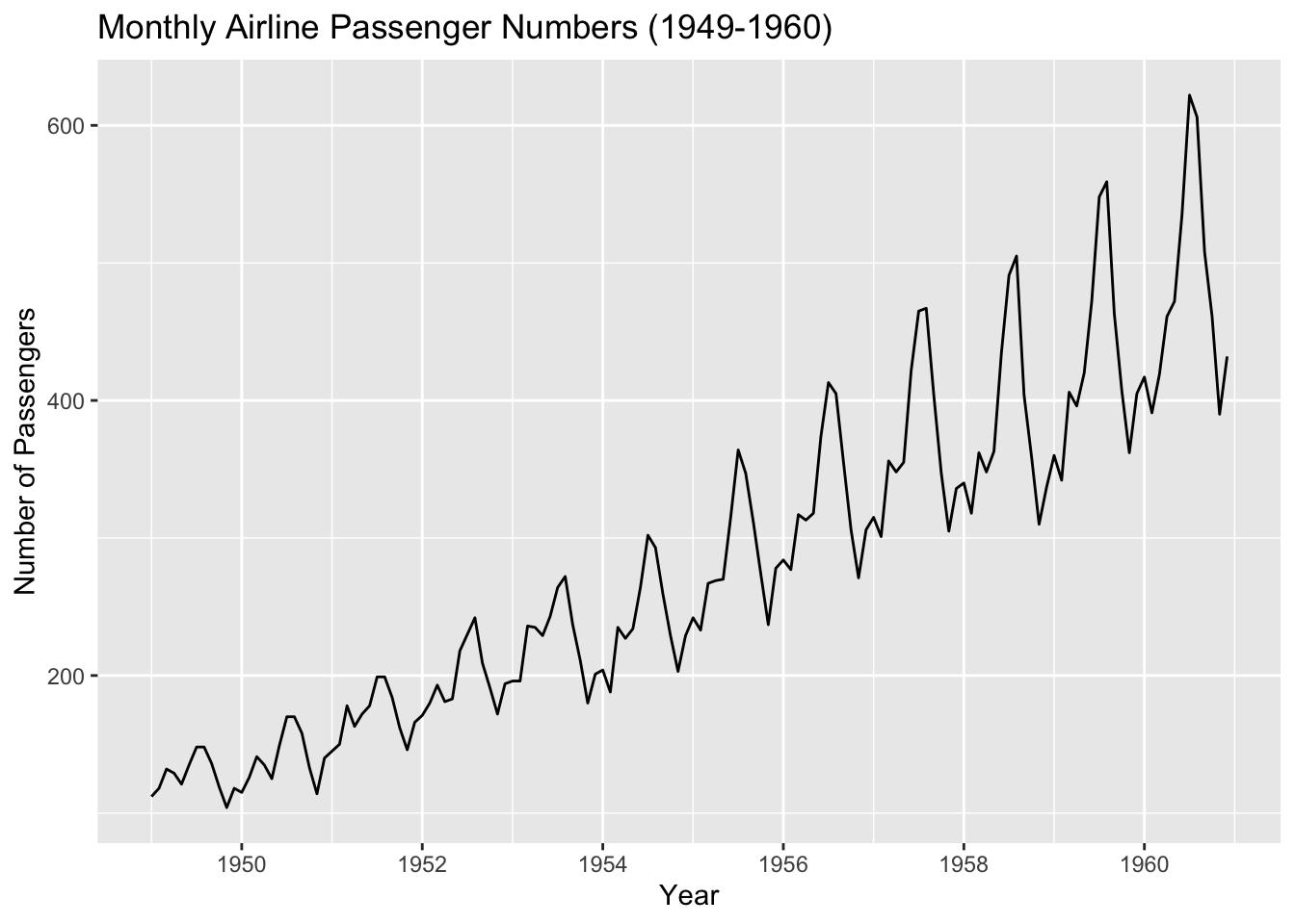
For example, here’s a raw time series of monthly airline passengers:
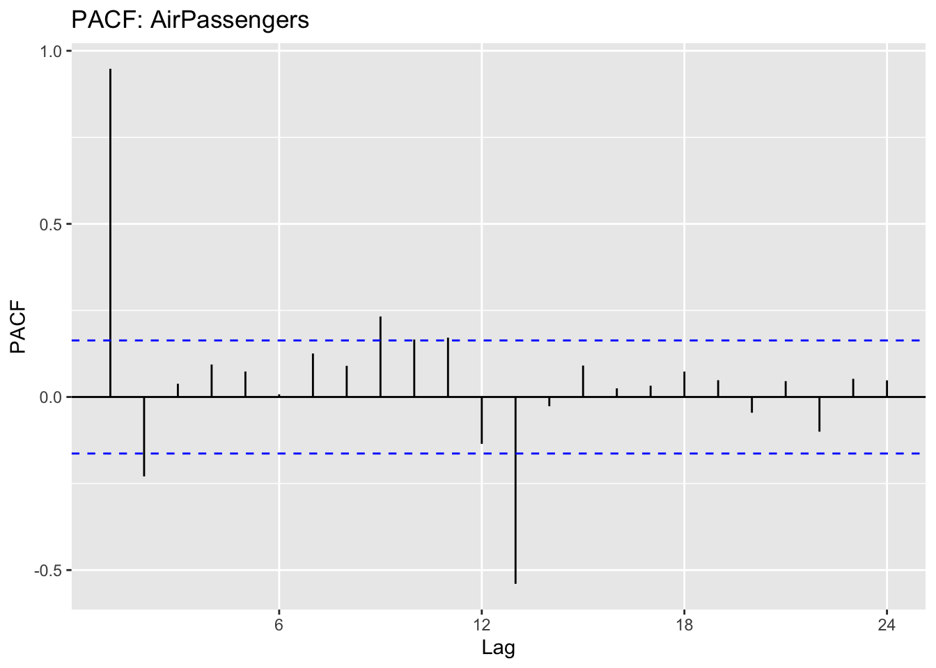
We can plot the ACF and the PACF for that time series:
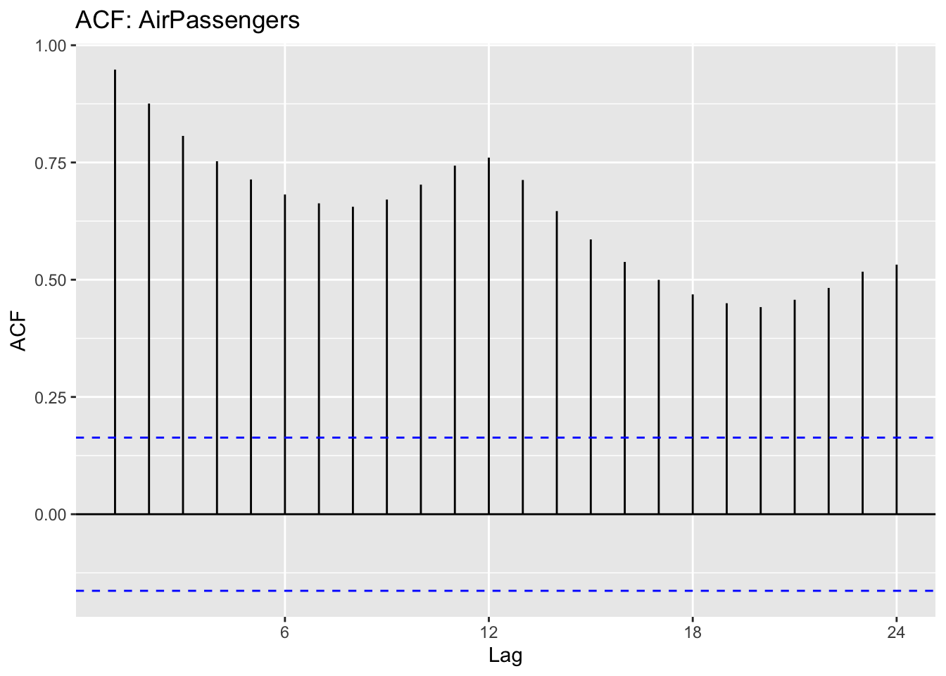
The ACF shows us how each value in the series is correlated with its past values.
The PACF helps identify the specific lag(s) contributing to the correlation.
Now, we need to interpret those plots to determine values for \(d\) and \(p\).
16.3.1 Step 1: Determining 𝑑 (differencing) using the ACF
The parameter 𝑑 represents the number of times we need to difference the series to make it stationary (i.e., remove trends and make the mean stable over time).
Remember: a stationary series has no obvious trend and has constant variance.
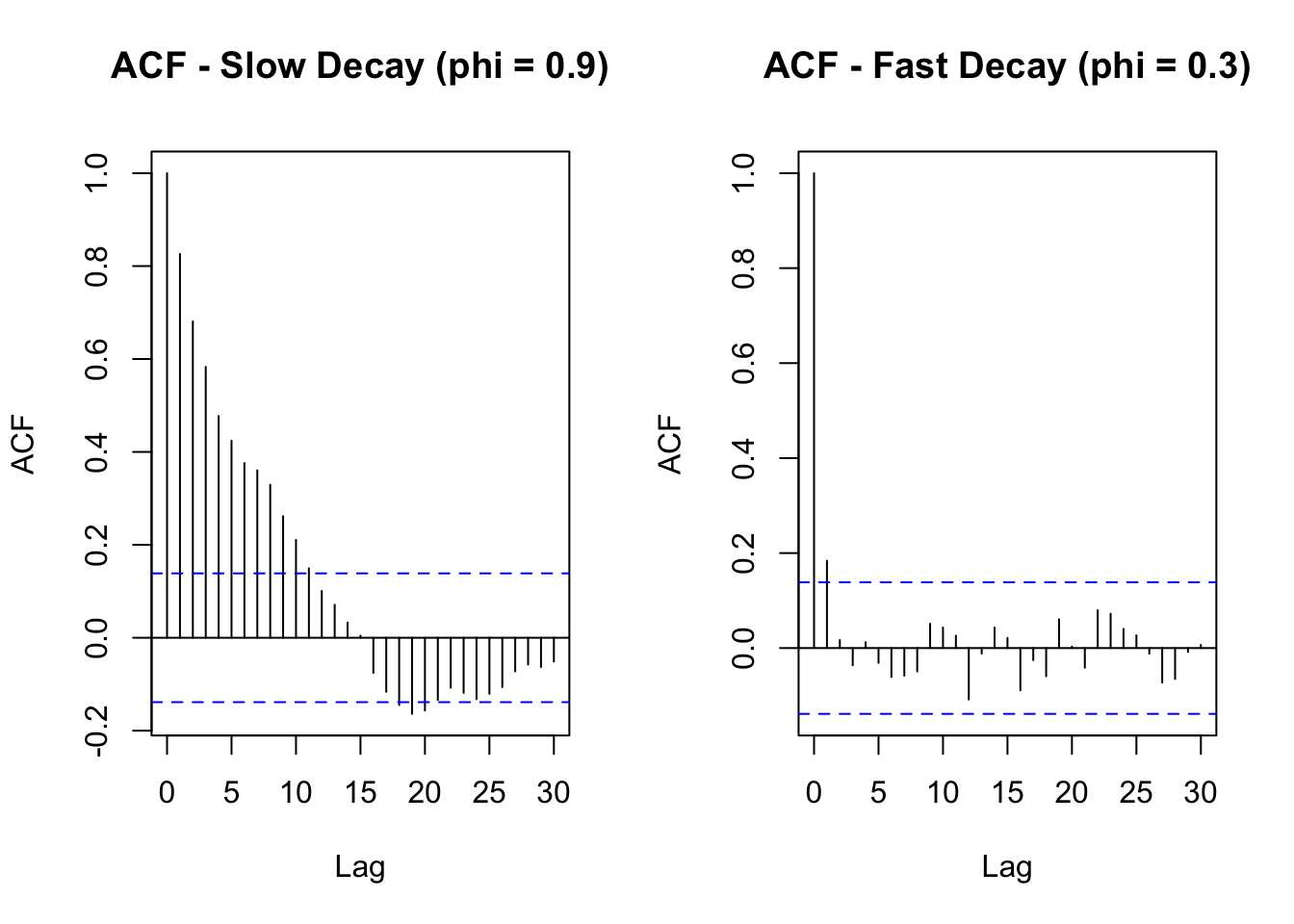
If the ACF shows a slow decay (gradual decrease over many lags), the series is non-stationary and needs differencing.
If differencing once (i.e., using first differences) makes the ACF decay quickly, 𝑑=1 is enough.
If the series is still non-stationary after one difference, try another difference, 𝑑=2 (but rarely more than this).
To check if differencing is needed:
Plot the ACF of the raw data. If it drops off very slowly, apply differencing.
Replot the ACF after differencing once. If the series is now stationary (ACF cuts off quickly), 𝑑=1
Look at the following plots. The one on the left has a slow decay while the one on the right has a fast decay. We would take a slow decay as a sign that differencing is required.
16.3.2 Step 2: Choosing 𝑝 (Autoregressive Order) using PACF
Once the series is stationary (after differencing 𝑑 times), we can use the Partial Autocorrelation Function (PACF) to determine 𝑝.
The PACF measures the direct relationship between a time point and its past values, removing effects from other intermediate lags.
If the PACF cuts off sharply after lag 𝑘(i.e., drops close to zero), then 𝑝=𝑘
If the PACF decays gradually, a higher 𝑝 may be needed.
General Rules:
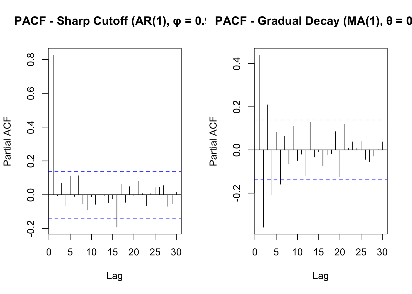
If PACF has a sharp cutoff at lag 𝑘, choose 𝑝=𝑘 (suggests an AR(𝑝 p) process).
If PACF declines gradually but ACF cuts off sharply, this suggests using an MA(𝑞) process instead.
If both ACF and PACF decay slowly, the data is not yet stationary; increase 𝑑.
Here are two plots showing a sharp cutoff in PACF, verus a slower (gradual) decay:
16.4 When to use ARIMA
ARIMA is best applied when:
- The data are (or can be made) stationary.
- Remember: “stationary” means the statistical properties (mean, variance) do not change over time. Sometimes differencing (the “I” part) is necessary to achieve stationarity.
- The series does not exhibit strong seasonal patterns (although there is an extension, SARIMA, which handles seasonality).
- We have a moderately large time series (enough data points to capture patterns in past values and forecast errors).
- We want a straightforward, well-established model that balances interpretability with reasonable forecasting performance.
16.5 Demonstration: Fitting and Forecasting with ARIMA
This may seem quite complex. Thankfully, R has a function called auto.arima() (part of the forecast package) that automates much of the decision-making.
Below is a simple demonstration of what auto.arima() produces when asked to automatically select the best ARIMA model, based on the AirPassengers data:
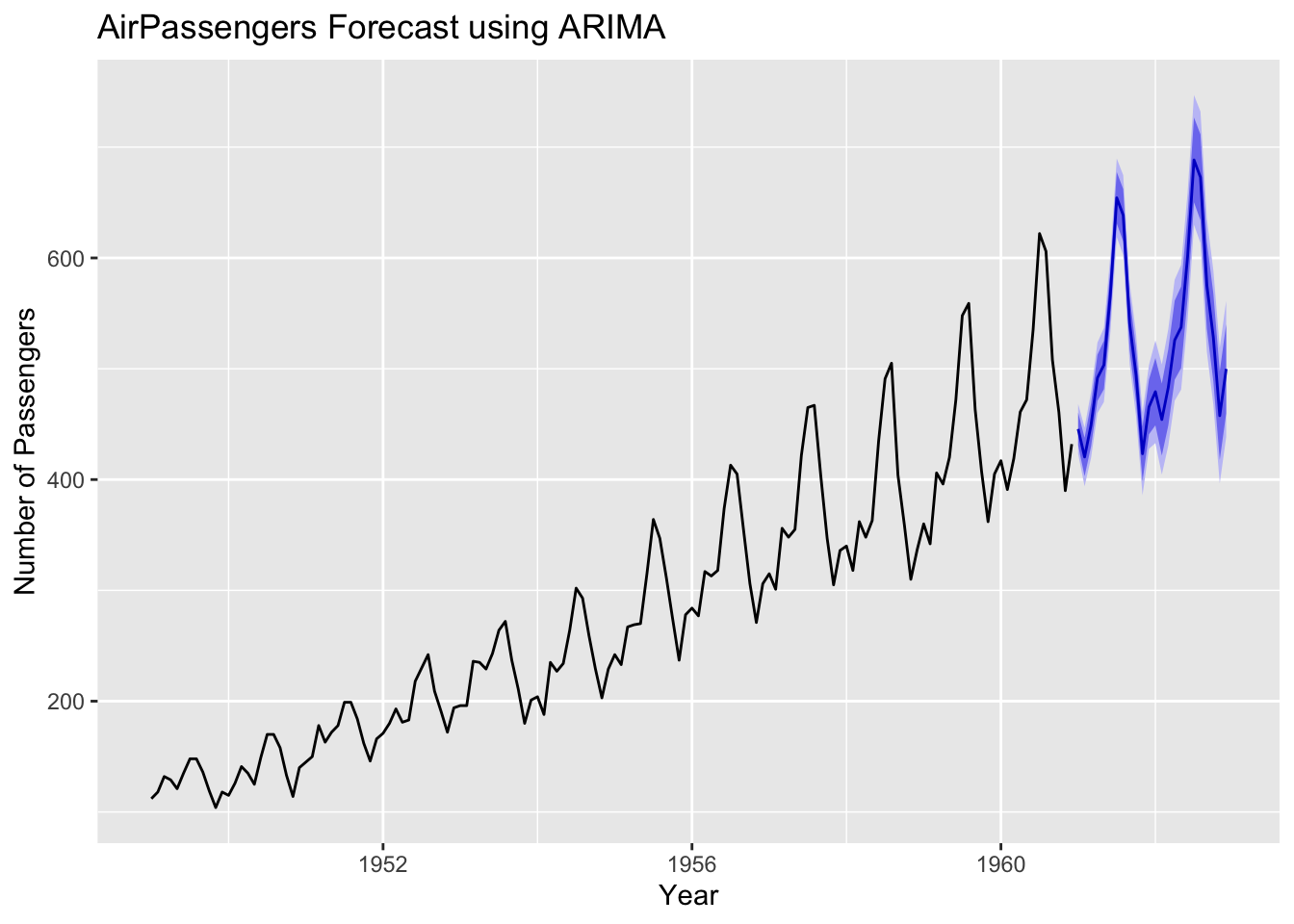
auto.arima() will look at the data, difference it if needed, and determine suitable \(p\), \(d\), \(q\) automatically.
We can examine the output of summary(fit) to see which ARIMA parameters were selected and how the model performed on this dataset.
16.5.1 Model selection criteria: AIC and BIC
Even with the help of ACF, PACF, and stationarity tests, we may still have more than one possible ARIMA model.
To choose the best one, we can compare their AIC (Akaike Information Criterion) and BIC (Bayesian Information Criterion):
- The AIC balances model fit with the number of parameters used. A lower AIC means a more efficient model.
- The BIC is similar to AIC, but with a stronger penalty for more parameters (this helps guard against overfitting).
Note: If model 1 has the lower AIC (and/or BIC), that suggests it might be the better choice. If model 2 is lower, that suggests it may offer a better trade-off between fit and complexity.
16.6 Parameter Estimation
16.6.1 Introduction
Once you’ve chosen an ARIMA model structure (defined by 𝑝, 𝑑, 𝑞), the next step is to estimate its parameters. These parameters include:
- Autoregressive coefficients (for the AR part);
- Moving Average coefficients (for the MA part);
- The intercept (if present); and
- Variance of residuals (error term).
The goal is to find parameter values that make the model fit the data well, without fitting it so closely that it performs poorly on unseen data.
16.6.2 Maximum likelihood estimation (MLE)
Maximum Likelihood Estimation (MLE) is a commonly-used method for estimating ARIMA parameters. It works by finding the parameter values that maximise the probability of observing the actual data.
In practice, statistical software like R uses iterative algorithms (like numerical optimisation) to adjust parameters and maximise the likelihood function.
MLE seeks a balance between fitting the data and recognising random noise.
Series: ts_data
ARIMA(1,1,1)

Coefficients:
          ar1     ma1
      -0.4742  0.8635
s.e.   0.1159  0.0720

sigma^2 = 975.8:  log likelihood = -694.34
AIC=1394.68   AICc=1394.86   BIC=1403.57

Training set error measures:
                   ME     RMSE      MAE       MPE     MAPE      MASE       ACF1
Training set 1.920932 30.91123 24.12171 0.4150816 8.566124 0.7530902 0.03750378
Note: - This output shows the estimated AR(1) and MA(1) coefficients, along with statistics like the log-likelihood, AIC, and BIC.
16.6.3 Least Squares for AR and MA Terms
For autoregressive (AR) models, Least Squares is a simple estimation method. It minimises the sum of squared errors between the model’s predictions and actual values.
In a purely AR model (e.g., AR(1) or AR(2)), this is straightforward:
The model predicts \(X_t\) using past values \(X_t-1, X_t-2,...\)
Minimising squared errors ensures the best-fitting line through past observations.
For moving average (MA) terms, Least Squares is more complex since errors depend on previous residuals. Many software packages use Conditional Sum of Squares (CSS), often combined with Maximum Likelihood Estimation (MLE) for parameter estimation.
This produces output like the following:
Series: ts_data
ARIMA(1,1,1)

Coefficients:
          ar1     ma1
      -0.4828  0.8751
s.e.   0.1137  0.0675

sigma^2 = 975.6:  log likelihood = -694.54

Training set error measures:
                   ME     RMSE      MAE       MPE   MAPE      MASE       ACF1
Training set 1.901601 30.90734 24.10162 0.3993277 8.5458 0.7524631 0.03549468
Note:
CSS minimises squared errors conditionally, using prior residual estimates.
While CSS and MLE can yield similar results, MLE is typically preferred if it converges well.
16.6.4 Overfitting vs. underfitting
You’ll remember from previous sections that overfitting happens when a predictive model fits noise in the historical data rather than the true underlying pattern. It gives us a model that is ‘too good’ to be applied to future data.
Signs of overfitting include:
- Very high accuracy on the training data but poor forecast performance on new or test data.
- Parameters that become too large or unstable.
‘Underfitting’ occurs when a model is too simple to capture important structure in the data. This can lead to:
- Systematic errors in forecasts, such as persistent bias or missed trends.
- Balancing Overfitting and Underfitting
We can use information criteria like AIC and BIC to compare models. Lower values generally indicate a better fit- to-complexity balance.
We can evaluate forecasts on a ‘hold-out’ or test set to check how well the model generalises to unseen data.
16.6.5 Summary
- Parameter Estimation is about finding the best ARIMA coefficients that represent the data’s patterns.
- Maximum Likelihood Estimation (MLE) is a standard method for ARIMA, aiming to maximise the probability of observing the actual data.
- Least Squares (CSS) can be applied for AR and MA terms, though it may be more approximate.
- Avoid overfitting by monitoring AIC, BIC, or forecast performance on new data.
- Underfitting can happen if the model is too simple and fails to capture important time series characteristics.
16.7 Model Diagnostics
16.7.1 Introduction
Once an ARIMA model has been fitted, we need to check how well it represents the data.
As in other forms of predictive modelling (like Discriminant Analysis), model diagnostics focus on assessing the residuals (the differences between predictions and actual values) and ensuring that they behave like white noise. If the residuals still contain patterns or correlations, it suggests our model may be missing key information.
16.7.2 Residual analysis for model adequacy
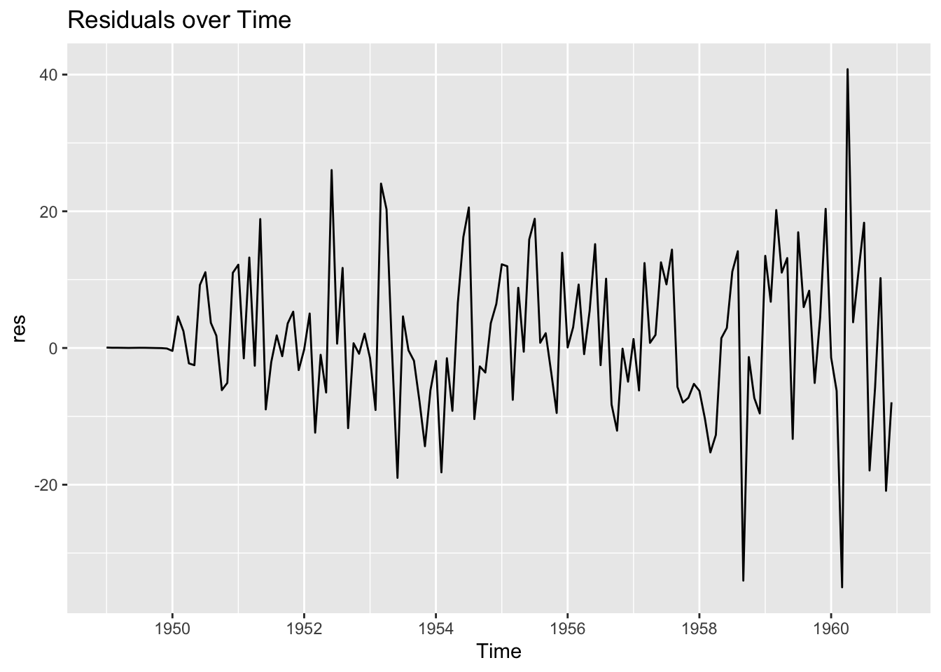
Residuals should look like a random scatter around zero, with no obvious trends or recurring patterns.
Remember: residuals are the differences between the predicted and the actual values.
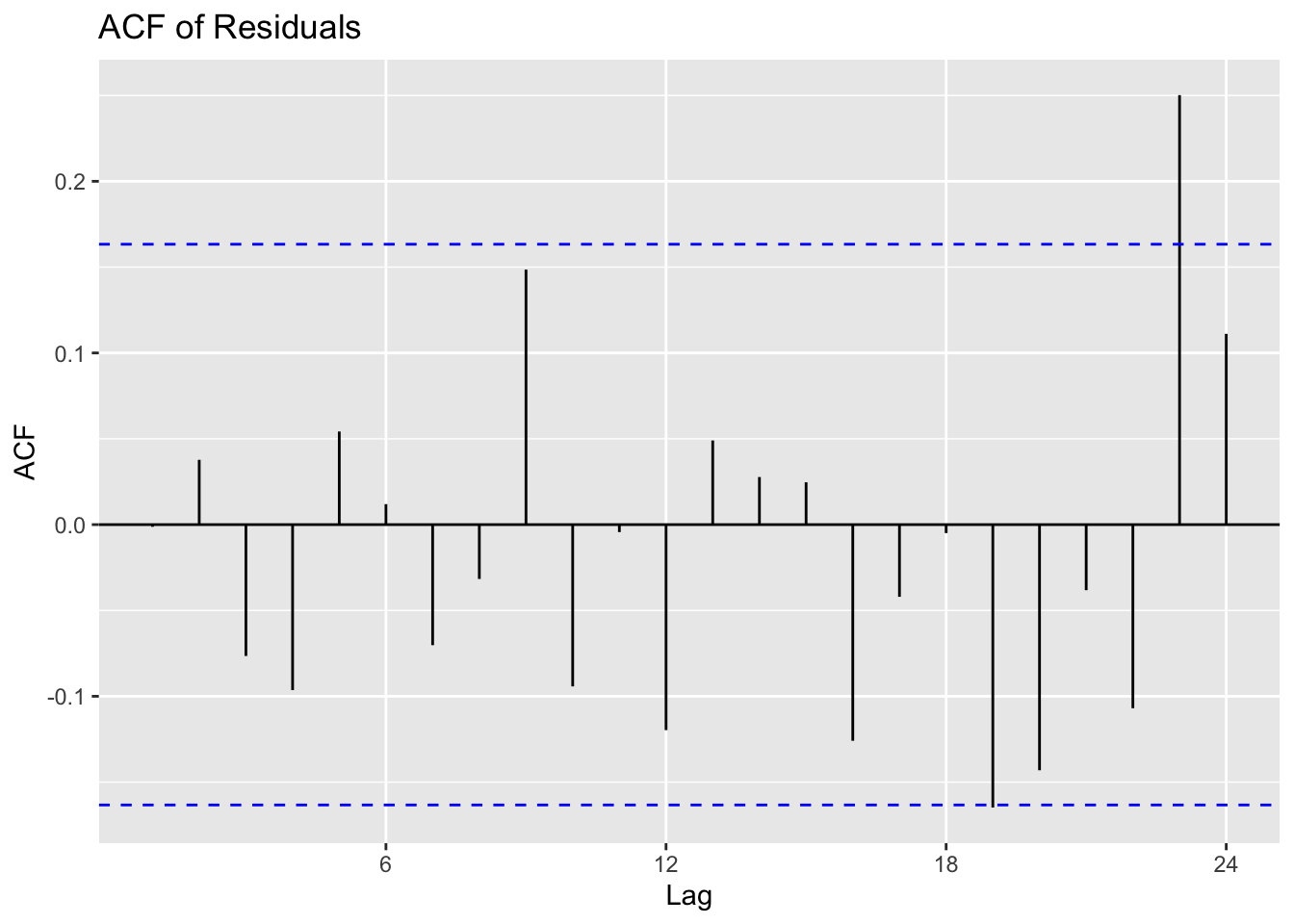
A good first step is to produce a time series plot of residuals, an autocorrelation function (ACF) plot, and a histogram to see if the errors roughly follow a normal distribution. If there are large spikes in the ACF or strong trends in the residual series, it indicates the model is not adequately capturing all the patterns in the data.
     Min.   1st Qu.    Median      Mean   3rd Qu.      Max.
-35.01381  -5.14754   0.02474   1.34231   8.90578  40.78953
Note: By examining these plots and summaries, we can often spot problems such as non-stationarity, missed seasonality, or an outlier event that heavily influences the model.
16.7.3 Ljung-Box Test for white noise
The Ljung-Box test is a more formal way of checking whether there is significant autocorrelation in the residuals.
If the residuals truly behave like white noise, the Ljung-Box test should return a high p-value, indicating no significant autocorrelation remains.
# Perform Ljung-Box test

Box.test(res, type = "Ljung-Box", lag = 10)
    Box-Ljung test

data:  res
X-squared = 8.6878, df = 10, p-value = 0.562
Note: A low p-value (e.g., below 0.05) suggests the presence of autocorrelation in the residuals, implying that the model can still be improved. A high p-value indicates the errors are essentially random, which is what we want for a well-fitted ARIMA.
16.7.4 Forecast Accuracy Metrics (RMSE, MAPE)
To further evaluate an ARIMA model, consider forecast accuracy metrics such as Root Mean Squared Error (RMSE) and Mean Absolute Percentage Error (MAPE).
RMSE measures the average magnitude of the residuals in the same units as the data;
MAPE shows the average percentage difference between the predicted and actual values.
These metrics can be useful for comparing multiple models.
Attaching package: 'Metrics'The following object is masked from 'package:forecast':
accuracy[1] 10.84619[1] 0.02800458Note: A lower RMSE or MAPE generally signals a better model fit, but it’s also important to avoid overfitting by introducing too many parameters. Balancing diagnostic checks and forecast accuracy ensures the model is neither underfitted nor overly complex.
16.8 Extensions of ARIMA
16.8.1 Introduction
As we’ve learned, ARIMA is a powerful time series forecasting method. However, real-world data often exhibit complexities such as strong seasonality or relationships to external factors that make its application problematic.
In this final section, we’ll explore advanced variations of ARIMA that address these more complex scenarios. Each method extends the core principles of ARIMA, allowing for nuanced modelling of patterns in the data.
16.8.2 Seasonal ARIMA (SARIMA) for Seasonal Patterns
Seasonal ARIMA, often denoted as SARIMA, is designed for data that show repeating patterns every certain number of observations, such as monthly sales or annual climate data.
SARIMA introduces additional seasonal components - ( 𝑃 , 𝐷 , 𝑄 ) - to account for seasonal autoregression, differencing, and moving average effects at a specific seasonal period 𝑠.
# Example of fitting a seasonal ARIMA to monthly data (AirPassengers)
sarima_fit <- auto.arima(AirPassengers, seasonal = TRUE)
summary(sarima_fit)
Series: AirPassengers
ARIMA(2,1,1)(0,1,0)[12]
Coefficients:
ar1 ar2 ma1
0.5960 0.2143 -0.9819
s.e. 0.0888 0.0880 0.0292
sigma^2 = 132.3: log likelihood = -504.92
AIC=1017.85 AICc=1018.17 BIC=1029.35
Training set error measures:
ME RMSE MAE MPE MAPE MASE
Training set 1.342306 10.84619 7.867539 0.4206996 2.800458 0.245628
ACF1
Training set -0.001248451# Plot forecast
sarima_forecast <- forecast(sarima_fit, h = 24)
autoplot(sarima_forecast) +
ggtitle("Seasonal ARIMA Forecast for AirPassengers")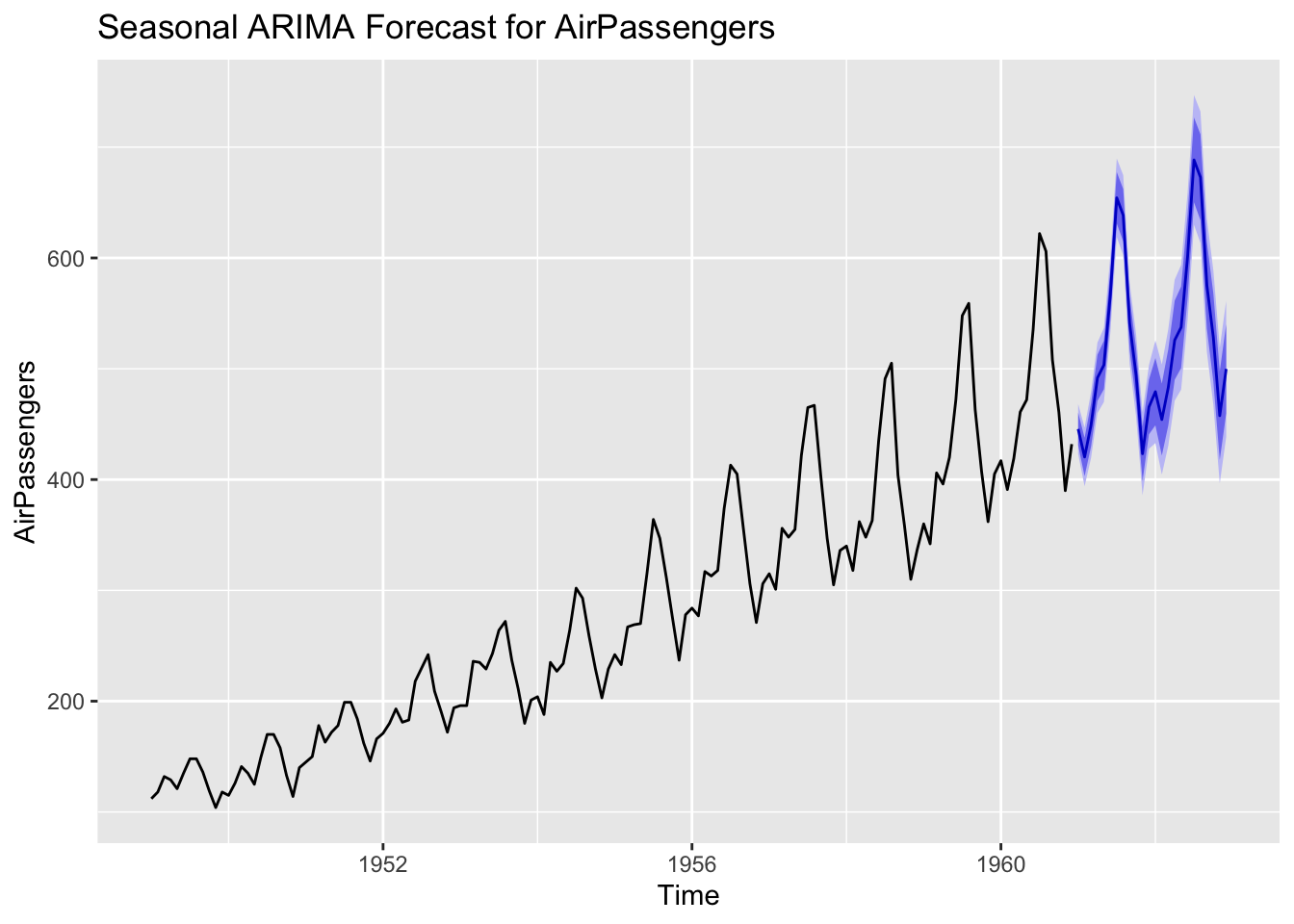
Seasonal differencing (the 𝐷 parameter) removes seasonal trends, while the seasonal AR and MA terms ( 𝑃 and 𝑄) capture persistent seasonal dependencies beyond the standard AR and MA components.
16.8.3 ARIMAX: ARIMA with exogenous variables
An ARIMAX (or ARIMA with eXogenous variables) model allows you to include additional predictor variables in the forecast.
Examples might include economic indicators when forecasting sales or climate variables when predicting energy consumption. The underlying ARIMA structure still models autocorrelations, but the exogenous factors can improve accuracy by capturing external influences.
Series: AirPassengers
Regression with ARIMA(2,1,1)(0,1,2)[12] errors

Coefficients:
         ar1    ar2      ma1     sma1    sma2     xreg
      0.5686  0.264  -0.9822  -0.1194  0.1601  -0.0666
s.e.  0.0894  0.093   0.0287   0.0983  0.0944   0.0651

sigma^2 = 129.9:  log likelihood = -502.46
AIC=1018.91   AICc=1019.82   BIC=1039.04

Training set error measures:
                   ME     RMSE      MAE       MPE     MAPE      MASE
Training set 1.307232 10.61922 7.641068 0.4008847 2.704432 0.2385575
                     ACF1
Training set -0.008620921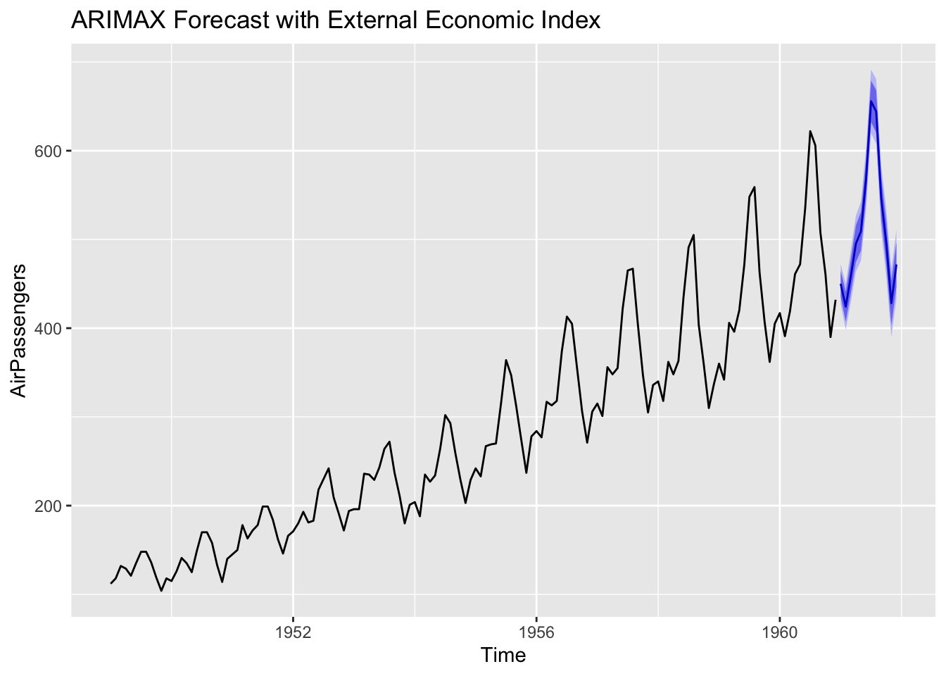
Including relevant external data can provide more accurate or more interpretable forecasts, especially if strong causal relationships exist between the time series and the exogenous predictor.
16.8.4 Hybrid Models - Combining ARIMA with Machine Learning
In some cases, combining ARIMA with machine learning techniques gives better forecasts, especially for complex datasets. A hybrid model might, for instance, first apply ARIMA to capture linear components, and then pass the residuals to a machine learning algorithm (like a neural network or a gradient boosting model) to capture any remaining nonlinear patterns.
By splitting linear and nonlinear tasks, hybrid models can outperform standard ARIMA, particularly in contexts with intricate dynamics. However, they can also become more complex to maintain and interpret.
We’ll cover these complex models towards the end of the module.